(EDA Part-2) First Look at the Titanic Dataset — Loading Data and Understanding Big 5

In Part 1, we compared EDA to a doctor’s examination. Now let’s actually open the patient file.

We’ll use the Titanic dataset from Kaggle. To follow along:

1. Go to kaggle.com/competitions/titanic/data
2. Download train.csv using link https://www.kaggle.com/competitions/titanic/data?select=train.csv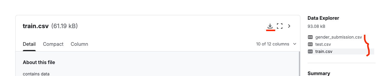
   
3. OpenOr open a free Kaggle Notebook — no install needed, runs in the browser

---

The analogy before we start — first day at a new job

Imagine you’ve just joined a company and someone hands you a stack of 891 employee files. You don’t start reading every file cover to cover. You first:

• Count how many files there are
• Look at the folder structure
• Check if any files are missing pages
• Scan a few at random to understand the format

That’s exactly what we do in this section. We’re not analysing anything deeply yet — we’re orientating ourselves.

---

The Quick-Start Routine

The following 5 commands are my non-negotiables. I run them on every single new dataset before doing anything else. No exceptions.

The Big 5 — run these on EVERY new dataset

print("Shape:", df.shape) # Returns (rows, columns)
print("\nData types:\n", df.dtypes) # Check if numbers are actually stored as numbers
print("\nFirst 5 rows:\n", df.head()) # View the first 5 rows
print("\nStatistical summary:\n", df.describe()) # Get a bird's-eye view of the math behind your data
print("\nNull values:\n", df.isnull().sum()) # The "Missing Data Report"

Step 0: import required library and load the dataset.

import pandas as pd
import numpy as np

# Load the dataset
df = pd.read_csv('train.csv')

Step 1: Shape

Definition: This attribute returns a tuple representing the dimensionality of the DataFrame. It tells you exactly how many rows (observations) and columns (features) are in your dataset.

Why it matters: It’s the very first step to understand the scale of your project. If you expect 10,000 rows but see only 100, you know something went wrong during data loading.

df.shape

Output:

Shape: (891, 12)

(891, 12) means 891 rows and 12 columns.

Step 2: dtypes

Definition: This property returns the data type (e.g., int64, float64, object) of each column.

Why it matters: It helps you identify Type Mismatches. For example, if a Price column is listed as an object (string) instead of a float, you won’t be able to perform math on it until it’s converted.

df.dtypes

Output:

Data types:
 PassengerId      int64
 Survived         int64
 Pclass           int64
 Name            object
 Sex             object
 Age            float64    # ← float means decimal values AND possibly nulls
 SibSp            int64
 Parch            int64
 Ticket          object
 Fare           float64
 Cabin           object
 Embarked        object

Watch out: Age is stored as float64, not int64. In pandas, an integer column with even ONE null value automatically becomes float64. That little decimal point is a hint telling you “this column has missing values.” Age should logically be whole numbers — the float is a red flag.

Step 3: head()

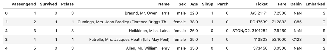
Definition: This method returns the first n rows (default is 5) of the dataset.

Why it matters: It’s a sanity check. It allows you to see the actual content of the cells, verify that headers are correct, and get a feel for how the data is formatted.

df.head()

Output:

Step 4: describe()

Definition: This method generates descriptive statistics that summarize the central tendency, dispersion, and shape of a dataset’s distribution (excluding NaN values).

Why it matters: In one command, you get the Mean, Standard Deviation, Min/Max, and Quartiles. It is the fastest way to spot outliers—if the Max value for age is 200, you’ve found a data entry error.

df.describe()

Output:

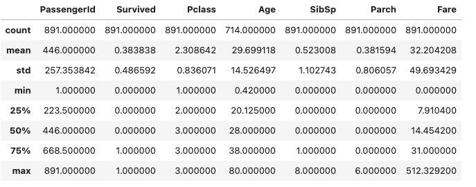
The df.describe() output looks scary but it’s just a table of 8 statistics per numeric column. Here’s what to focus on:

Age column — what the numbers say:

Stat	Value	What it means
count	714	Only 714 of 891 rows have an age recorded
mean	29.7 years	Average age of passengers with known age
std	14.5	Spread of ages — quite wide
min	0.42	There were infants on board!
50% (median)	28.0 years	Half of passengers were younger than 28
max	80.0	Oldest passenger was 80

Fare column — the red flag:

Stat	Value
mean	£32.20
median (50%)	£14.45
max	£512.33

Key insight: Mean (£32.20) is more than double the median (£14.45). When mean >> median, you have right skew — a few extremely expensive tickets are pulling the average way up. This matters when we build our model later, because many ML algorithms assume features are roughly normally distributed.

Let’s understand the meaning of these terms:
Mean (Average): The sum of all values divided by the total number of values. It is the most common measure of center but is highly sensitive to outliers (extreme values).

Median: The middle value when the data is sorted from smallest to largest. If there is an even number of observations, it is the average of the two middle numbers. Unlike the mean, the median is robust, meaning it isn’t easily skewed by a few very high or very low numbers.

Mode: The value that appears most frequently in a dataset. A dataset can have one mode, multiple modes (bimodal or multimodal), or no mode at all. This is particularly useful for categorical data (e.g., finding the most common car color in a dataset).

Standard Deviation (Std):
This measures the average distance of each data point from the mean.

• Low Std: Data points are close to the mean (the data is consistent).
• High Std: Data points are spread out over a wide range (the data is volatile).

In machine learning, standard deviation is used in feature scaling (like Standardization) to ensure that features with different scales (e.g., Age vs. Annual Income) don’t bias the model.

Term	What it tells you	Sensitivity to Outliers
mean	The mathematical center	High
median	The physical middle	Low
mode	The most popular value	Low
std	The “spread” or risk	High

---

Step 4.1: Check your categorical columns too

describe() only covers numeric columns by default. Don’t forget the string columns.

# Count unique values per categorical column
for col in ['Sex', 'Embarked', 'Pclass']:
    print(f"\n{col}:")
    print(df[col].value_counts())

Output:

Sex:
 male      577   # (64.7%)
 female    314   # (35.3%)

Embarked:
 S    644   # Southampton (UK)
 C    168   # Cherbourg (France)
 Q     77   # Queenstown (Ireland)
 NaN    2   # (missing — we'll fix this in Part 3)

Pclass:
 3    491   # lower class (55% of all passengers!)
 1    216   # upper class
 2    184   # middle class

Step 5: isnull().sum()

Definition: This is a chained command. isnull() creates a boolean mask (True/False) for missing values, and .sum() adds up those Trues for every column.

Why it matters: Missing data is the enemy of Machine Learning. This command creates a Missing Data Report, telling you exactly where the holes are so you can decide whether to fill them (imputation) or drop them.

df.isnull().sum()

Output:

PassengerId      0
Survived         0
Pclass           0
Name             0
Sex              0
Age            177
SibSp            0
Parch            0
Ticket           0
Fare             0
Cabin          687
Embarked         2
dtype: int64

---

What this already tells us — the iceberg analogy

Like the Titanic itself, we’re only seeing the surface so far. But even from these basic checks, we’ve already learned:

• 64% male passengers — the Titanic famously applied women and children first, so Sex is almost certainly a strong predictor
• 55% were in 3rd class — lower class passengers had less access to lifeboats
• Most boarded at Southampton — this could be correlated with class
• Age has 20% missing — we need a strategy beyond simple mean imputation

The iceberg analogy: EDA is already making us smarter before we write a single model line. We now have context — and context is how you catch the mistakes that plain accuracy scores hide.

---

Quick recap: what we found in 5 lines of code

Finding	What it means
Age stored as float	Has missing values — needs imputation
Fare: mean >> median	Right-skewed — consider log transform
Cabin: 687 nulls	77% missing — can’t impute, need different strategy
Sex: 64% male	Class imbalance in a key feature
Pclass 3: 55% of passengers	Most passengers were lower class

---

What’s next?

In Part 3, we plot distributions for every important column with histograms and box plots, understand what’s actually inside the Age and Fare distributions, and decide how to handle that 77% missing Cabin column.

That’s where the real visual EDA begins. See you there!